Demography data for IUSSI

In case of questions, please contact Biplabendu Das

---

What is this document?

The goal:

Perform a rapid exploratory analyses of the demography data obtained from the survey performed on the audience interested in or/and attending the upcoming IUSSI international conference in 2022, San Diego.

---

01 Raw data

Number of folks that took the survey: 226

Let’s take a look at few rows and columns of the raw data.

	time_of_entry	age	gender	add_gender	sex_orientation	add_sex_orientation	residence_location
10	2022/02/11 11:48:02 AM EST	25-29 years old	Cisgender man	NA	Heterosexual	NA	Continental US
11	2022/02/11 6:05:24 PM EST	25-29 years old	Cisgender woman	NA	Bisexual	NA	Continental US
12	2022/02/11 8:10:38 PM EST	35-39 years old	Cisgender woman	NA	Heterosexual	NA	Continental US
13	2022/02/13 12:12:18 PM EST	21-24 years olf	Cisgender man	NA	Homosexual (gay/lesbian)	NA	Europe

	research_location	ethnic_identity	add_ethnic_identity	religious_identity	add_religious_identity	disability_identity
10	Continental US	Southeast Asian;Brown	NA	I am not religious	NA	I have no disability/impairment
11	Australasia	Hispanic;Latinx;Brown	NA	Prefer not to respond	NA	NA
12	Continental US	Black	NA	Christianity	NA	I have no disability/impairment
13	Europe	White	NA	I am not religious	NA	I have no disability/impairment

What does each column contain?

Column name: Description

• time_of_entry:
• age:
• and so on..

---

02 Format data

Get the data into a tidy format

• remove columns that are not useful for a first assessment
  • time_of_entry
  • add_xxx (all columns that contain additional response not listed)
• format each column by
  • separating multiple choices into separate rows
  • factorizing the variables
  • checking for erronneous choices/inputs

## Tidy and save data
dat <- 
  
  raw.dat %>% as_tibble() %>% 
  
  
  ## remove columns that you do not want
  select(-time_of_entry) %>% 
  select(-starts_with("add")) %>% 
  
  ## add a unique ID for each person
  rownames_to_column("ID") %>% 
  
  ## AGE
  mutate(age = str_split_fixed(age, " ", n=2)[,1]) %>%
  mutate(age = ifelse(age %in% c("","Prefer"), other.var, age)) %>%
  mutate(age = as.factor(age)) %>%
      # ## Plot: AGE
      # group_by(age) %>%
      # summarise(num = n()) %>% 
      # ##
      # ggplot(aes(x=age, y=num)) +
      #   geom_point() +
      #   coord_flip() +
      #   theme_Publication()

  
  ## GENDER
    # there are two entries that contains the following two responses for gender identity
    # c("Cisgender woman;Prefer not to respond", "Transgender man;Cisgender woman")),
    # five entries that stated "Prefer not to respond", and one which is NA.
    # Rename all to "Other"
  mutate(gender = ifelse(!gender %in% c("Cisgender man", "Cisgender woman", "Non-binary",
                       "Transgender man", "Transgender woman"), other.var, gender)) %>%
  mutate(gender = as.factor(gender)) %>%
      # ## Plot: GENDER
      # group_by(gender) %>%
      # summarise(num = n()) %>%
      # na.omit() %>%
      # ##
      # ggplot(aes(x=gender, y=num/sum(num)*100)) +
      #   geom_point() +
      #   coord_flip() +
      #   theme_Publication()

  
  ## sex_orientation
  mutate(sex_orientation = ifelse(sex_orientation %in% c("Additional identity not listed? (Please click next and share)","Prefer not to respond"), other.var, sex_orientation)) %>% 
  mutate(sex_orientation = as.factor(sex_orientation)) %>% 
  
  
  ## residence_location
  mutate(residence_location = ifelse(residence_location %in% c("Central America;Other",
                                     "Continental US;South Asia",
                                     "Europe;Middle East",
                                     "Europe;Southeast Asia",
                                     "Other"), other.var, residence_location)) %>%
  mutate(residence_location = as.factor(residence_location)) %>% 


  ## research location
  # filter(research_location %in% c("Central America;Continental US", "Europe;South America")) %>%
  separate_rows(research_location, sep = ";") %>% 
  mutate(research_location = as.factor(research_location)) %>% 
  
  
  ## ethnic_identity
  separate_rows(ethnic_identity, sep = ";") %>% 
  mutate(ethnic_identity = ifelse(ethnic_identity %in% c("A race or ethnicity not listed",
                                                         "Prefer not to respond"), 
                                  other.var, ethnic_identity)) %>% 
  mutate(ethnic_identity = as.factor(ethnic_identity)) %>% 
  
  
  ## religious_identity
  mutate(religious_identity = ifelse(religious_identity %in% c("An additional affiliation not listed",
                                                               "Prefer not to respond"), 
                                     other.var, religious_identity)) %>% 
  mutate(religious_identity = as.factor(religious_identity)) %>% 
  
  
  ## disability_identity
  separate_rows(disability_identity, sep = ";") %>% 
  mutate(disability_identity = as.factor(disability_identity)) %>% 
  

  ## written_english
  mutate(written_english = as.factor(written_english)) %>% 
  
  
  ## spoken_english
  mutate(spoken_english = as.factor(spoken_english)) %>% 
  
  
  ## children_responsibility
  mutate(children_responsibility = as.factor(children_responsibility)) %>% 
  
  
  ## adult_responsibility
  mutate(adult_responsibility = ifelse(adult_responsibility %in% c("Prefer not to respond", "Other"),
                                       other.var, adult_responsibility)) %>% 
  mutate(adult_responsibility = as.factor(adult_responsibility)) %>% 
  
  
  ## funds_for_care_inhibit
  mutate(funds_for_care_inhibit = as.factor(funds_for_care_inhibit)) %>% 
  
  
  ## firstgen
  mutate(firstgen = as.factor(firstgen)) %>%  
  
  
  ## current position
  separate_rows(current_position, sep = ";") %>% 
  mutate(current_position = as.factor(current_position)) %>% 
  
  
  ## which_attended_before
  separate_rows(which_attended_before, sep = ";") %>% 
  mutate(which_attended_before = as.factor(which_attended_before)) %>% 

  
  ## role_attended_before
  separate_rows(role_attended_before, sep = ";") %>% 
  mutate(role_attended_before = as.factor(role_attended_before)) %>% 

  
  ## current_institute_desc
  separate_rows(current_institute_desc, sep = ";") %>% 
  mutate(current_institute_desc = as.factor(current_institute_desc)) %>% 
  
  
  ## barriers_what_degree
  mutate(barriers_what_degree = as.factor(barriers_what_degree)) %>% 
  
  
  ## barriers_which
  separate_rows(barriers_which, sep = ";") %>% 
  mutate(barriers_which = as.factor(barriers_which))


# ## get a glimpse of the tidy data
# dat[10:13,1:7] %>% 
#   kable() %>% 
#   kable_styling(bootstrap_options = c("striped"), full_width = F, position = "center", latex_options = "scaled_down")
# 
# dat[10:13,8:13] %>% 
#   kable() %>% 
#   kable_styling(bootstrap_options = c("striped"), full_width = F, position = "center", latex_options = "scaled_down")

---

03 Visualize

## Use this code chunk to define paramaters, such as color palettes and such

## COLOR
# role attended before
roles.color <- c("#005C53", "#F2E744", "#D9814E", "#BF6854", "#261B1A", "grey60")

Age & gender

## AGE + GENDER
dat %>% 
  
  # remove the rows with no age/gender info
  filter(age != other.var) %>% 
  filter(!is.na(gender)) %>%
  # filter(gender != "Other") %>% 
  
  # tally the number of people in a given age group for a given gender
  distinct(ID, age, gender) %>%
  group_by(age, gender) %>% 
  summarize(num=n()) %>% 
    
  ## Plot: AGE + GENDER
  ggplot(aes(x=age, y=num, fill=gender, group=gender)) +
    labs(y="number of people") +
    # geom_hline(yintercept = 5, col="grey60", alpha=0.7, size=1) +
    geom_bar(position="stack", stat="identity") +
    coord_flip() +
    theme_Publication() +
    scale_colour_Publication() +
    scale_fill_Publication() +
    guides(fill = guide_legend(nrow = 3))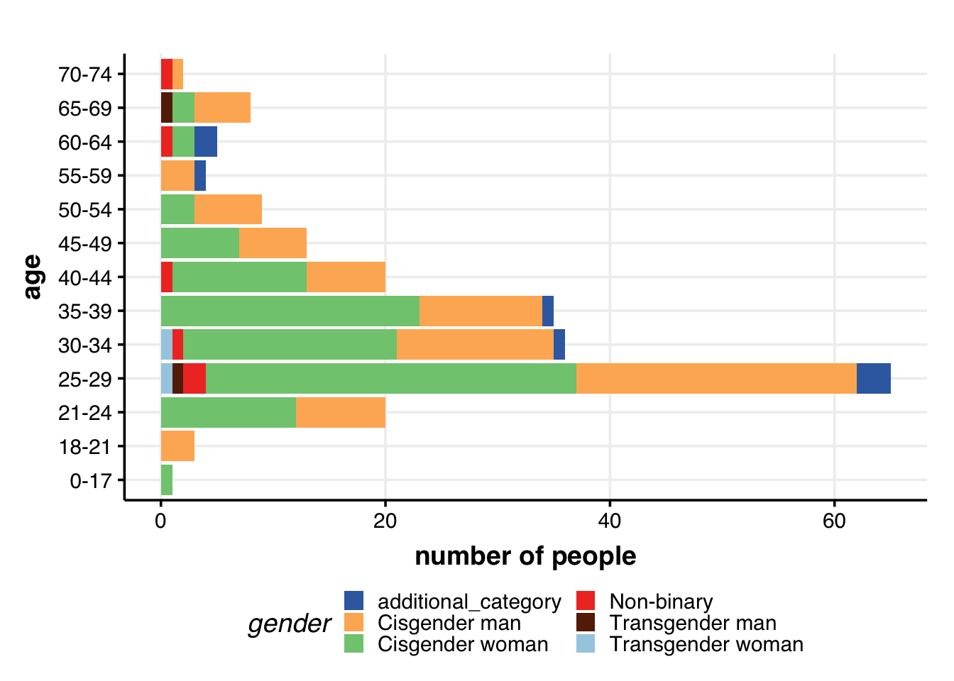

---

Residence location & gender

# Residence location & gender
dat %>%

  # filter(!residence_location %in% c("Other")) %>% 
  filter(!is.na(residence_location)) %>%
  filter(!is.na(gender)) %>%
  # filter(gender != "Other") %>% 
  
  distinct(ID, residence_location, gender) %>% 
  group_by(residence_location, gender) %>%
  summarize(num = n()) %>% 
  
  ggplot(aes(x=residence_location, y=num, fill=gender, group=gender)) +
    labs(y="number of people") +
    # geom_hline(yintercept = 5, col="grey60", alpha=0.7, size=1) +
    geom_bar(position="stack", stat="identity") +
    coord_flip() +
    theme_Publication() +
    scale_colour_Publication() +
    scale_fill_Publication() +
    guides(fill = guide_legend(nrow = 3))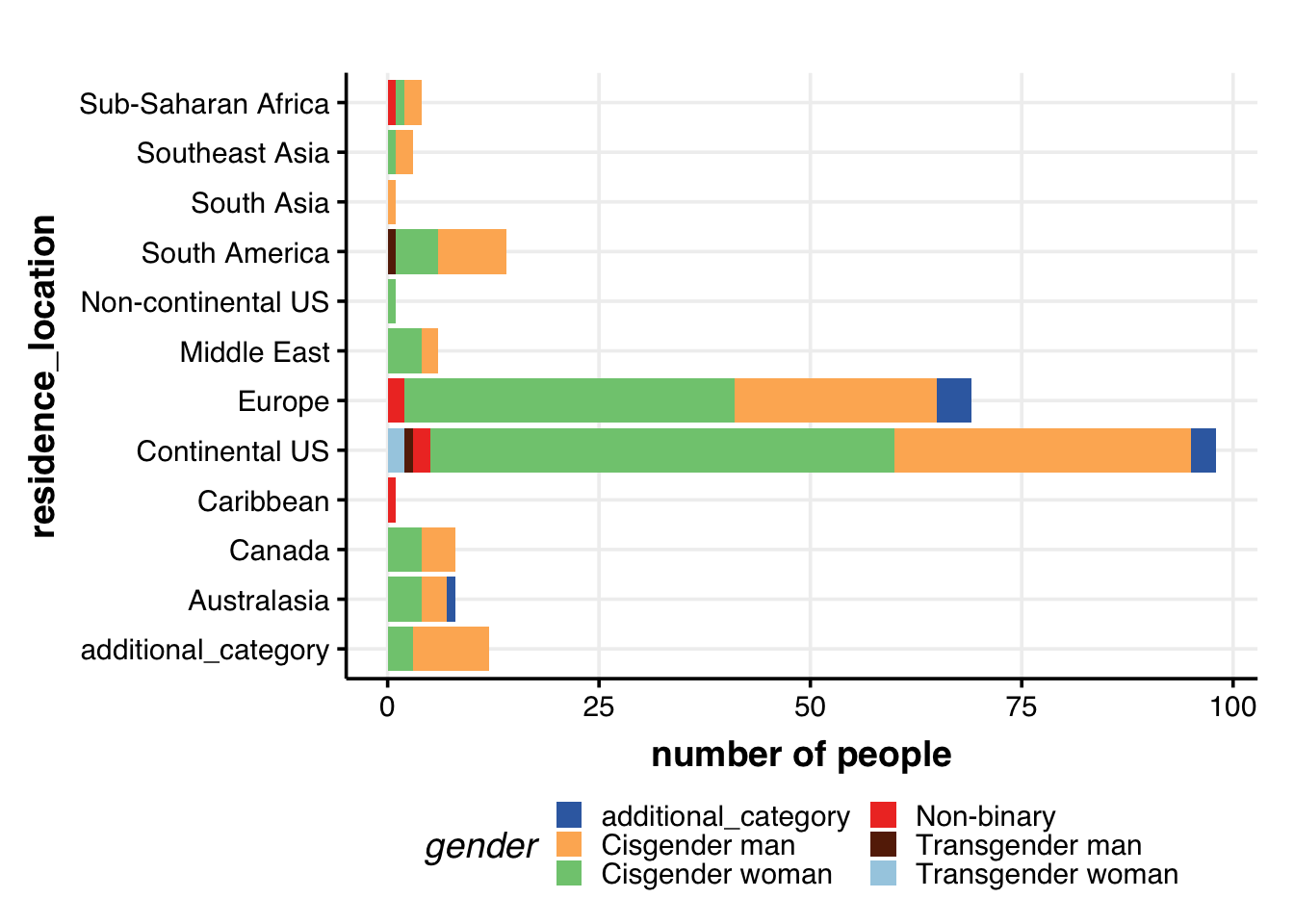

---

Research location & gender

## Plot: research_location + gender
dat %>% 
  
  filter(!is.na(research_location)) %>%
  filter(!is.na(gender)) %>%
  # filter(gender != "Other") %>%
  
  distinct(ID, research_location, gender) %>% 
  group_by(research_location, gender) %>%
  summarize(num = n()) %>% 
  
  ggplot(aes(x=research_location, y=num, fill=gender, group=gender)) +
    geom_bar(position="stack", stat="identity", size=2) +
    labs(y="number of people") +
    # geom_hline(yintercept = 5, col="grey60", alpha=0.7, size=1) +
    coord_flip() +
    theme_Publication() +
    scale_colour_Publication() +
    scale_fill_Publication() +
    guides(fill = guide_legend(nrow = 3))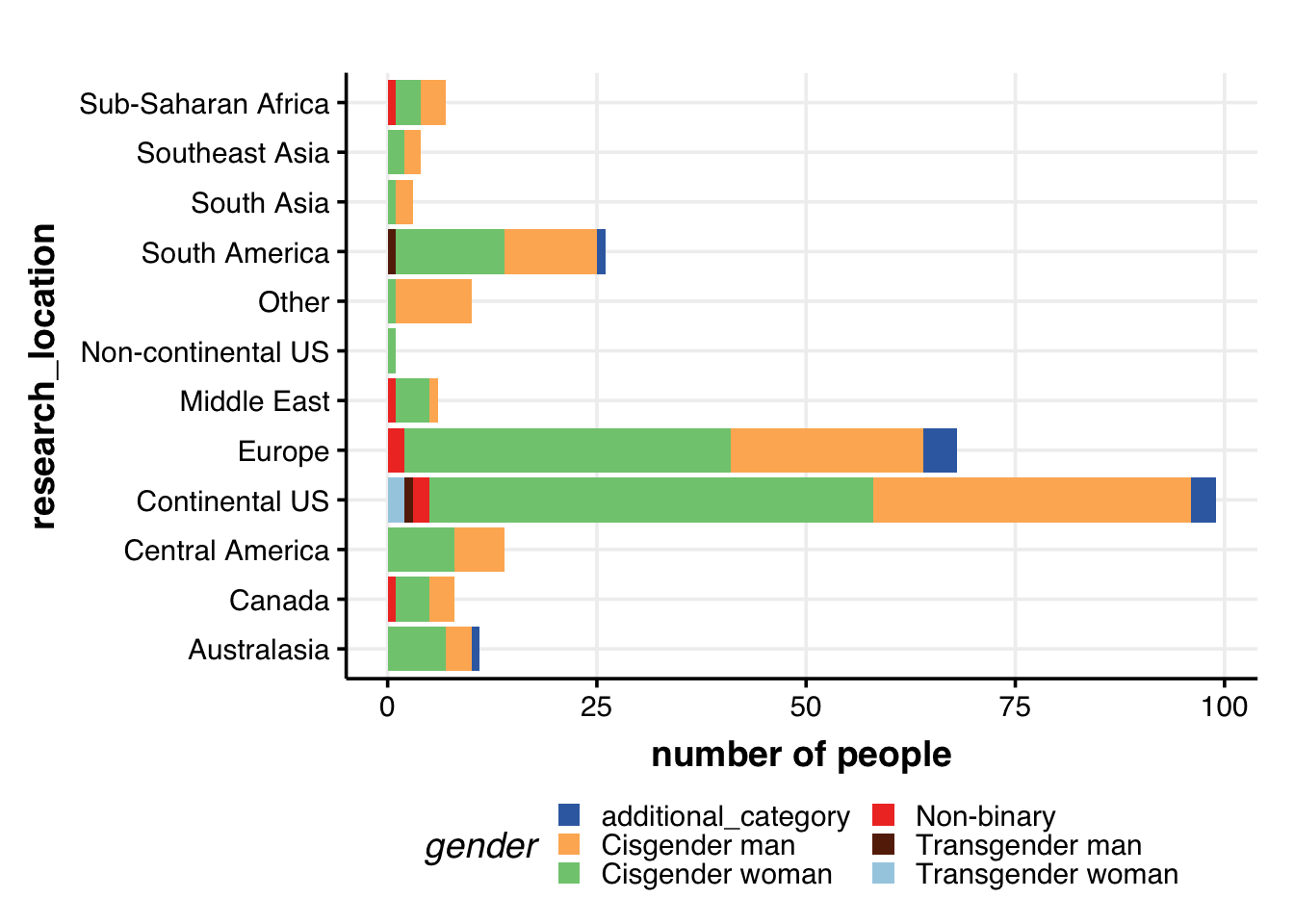

A bunch of folks perform research in Central America, but there seems to be no representation from folks living in Central America. There is, of course, the possibility that folks residing in Central America did not take the survey.

---

Role of attendee & gender

dat %>% 
  
  # remove the rows with no info
  filter(!is.na(role_attended_before)) %>%
  filter(!is.na(gender)) %>%
  # filter(gender != "Other") %>% 
  
  distinct(ID, role_attended_before, gender) %>% 
  group_by(role_attended_before, gender) %>%
  summarize(num = n()) %>% 
    
  ## Plot: research_location + gender
  ggplot(aes(x=role_attended_before, y=num, fill=gender, group=gender)) +
    geom_bar(position="stack", stat="identity", size=2) +
    labs(y="number of people") +
    # geom_hline(yintercept = 5, col="grey60", alpha=0.7, size=1) +
    coord_flip() +
    theme_Publication() +
    scale_colour_Publication() +
    scale_fill_Publication() +
    guides(fill = guide_legend(nrow = 3))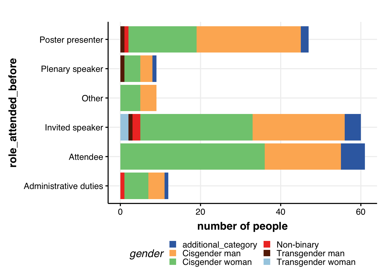

---

Current position & gender

dat %>% 
  
  filter(!is.na(current_position)) %>%
  filter(!is.na(gender)) %>%
  # filter(gender != "Other") %>% 

  distinct(ID, current_position, gender) %>% 
  group_by(current_position, gender) %>%
  summarize(num = n()) %>% 
  
  ggplot(aes(x=current_position, y=log2(num+1), fill=gender, group=gender)) +
    geom_bar(position="stack", stat="identity", size=2) +
    labs(y="number of people") +
    # geom_hline(yintercept = 5, col="grey60", alpha=0.7, size=1) +
    coord_flip() +
    theme_Publication() +
    scale_colour_Publication() +
    scale_fill_Publication() +
    guides(fill = guide_legend(nrow = 3))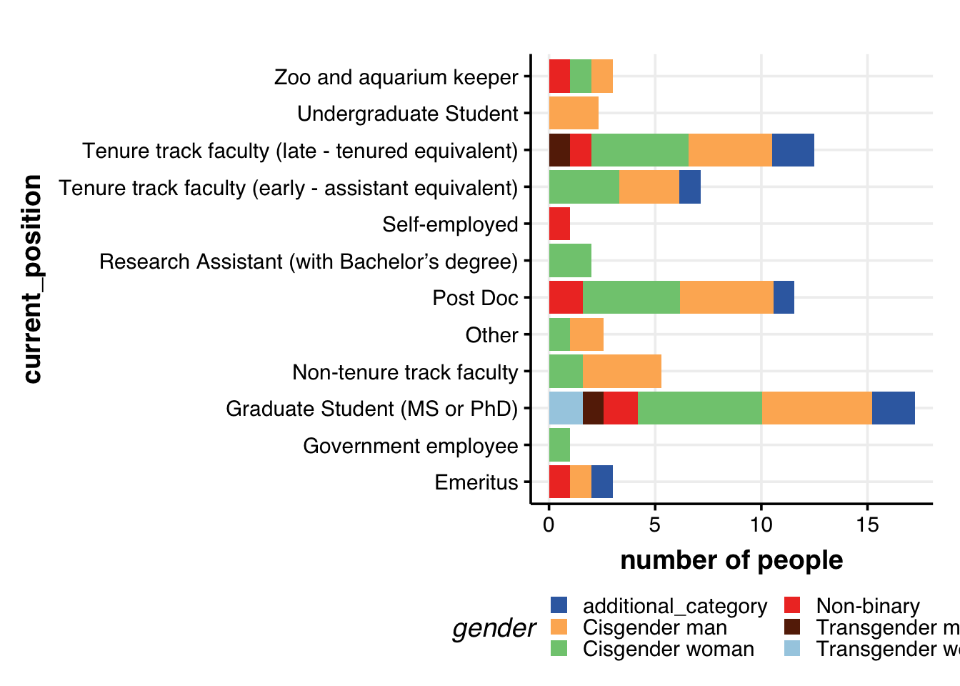

---

---

Role of attendee & residence location

dat %>% 
  
  # remove the rows with no age/gender info
  filter(!is.na(role_attended_before)) %>%
  filter(!is.na(residence_location)) %>%
  # filter(gender != "Other") %>% 
  
  distinct(ID, role_attended_before, residence_location) %>% 
  group_by(role_attended_before, residence_location) %>%
  summarize(num = n()) %>%
    
  ggplot(aes(x=residence_location, y=num, fill=role_attended_before, group=role_attended_before)) +
    geom_bar(position="stack", stat="identity", size=2) +
    labs(y="number of people") +
    # geom_hline(yintercept = 5, col="grey60", alpha=0.7, size=1) +
    coord_flip() +
    theme_Publication() +
    scale_colour_Publication() +
    # scale_fill_Publication() +
    scale_fill_manual(values = roles.color) +
    guides(fill = guide_legend(nrow = 3))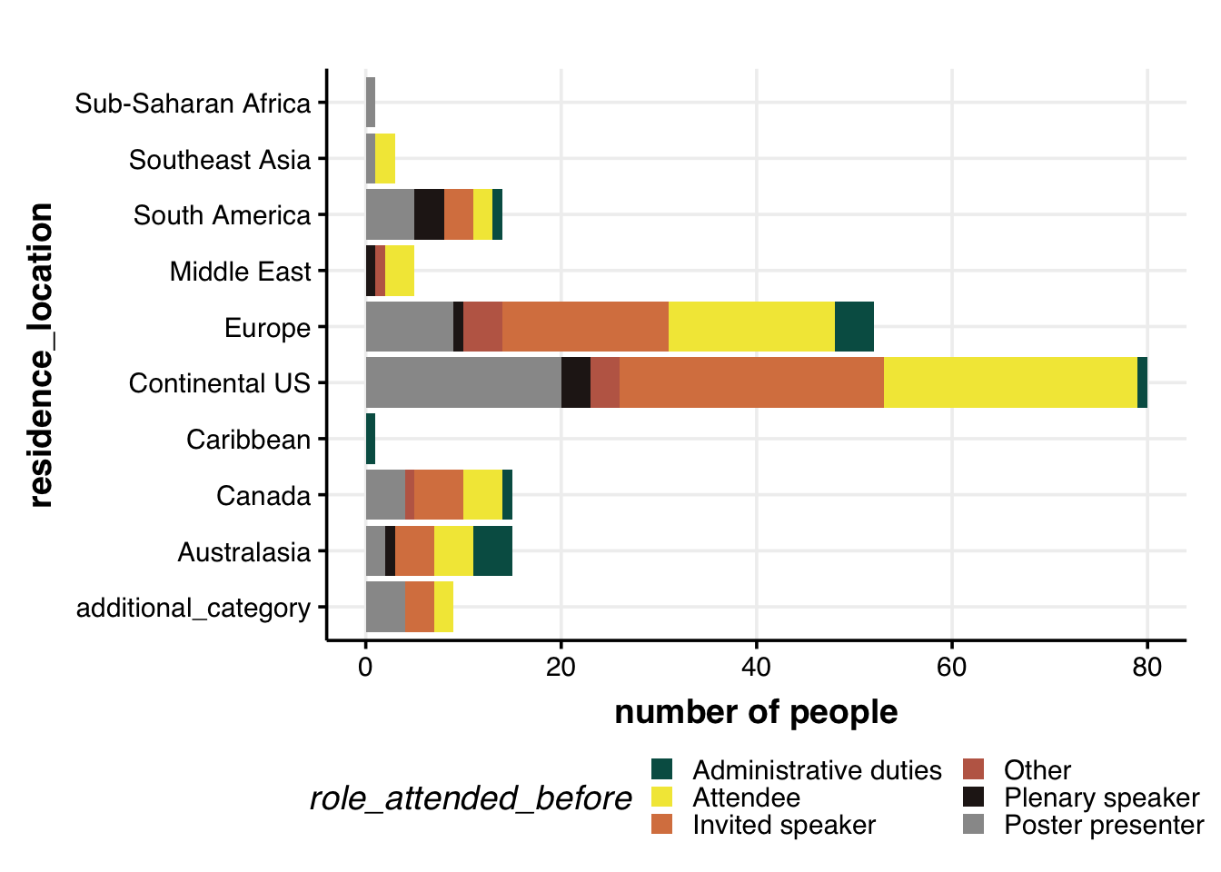

---

Role of attendee & current position

dat %>% 
  
  # remove the rows with no age/gender info
  filter(!is.na(role_attended_before)) %>%
  filter(!is.na(current_position)) %>%
  # filter(gender != "Other") %>% 
  
  distinct(ID, role_attended_before, current_position) %>% 
  group_by(role_attended_before, current_position) %>%
  summarize(num = n()) %>% 
    
  ## Plot: research_location + gender
  ggplot(aes(x=current_position, y=num, fill=role_attended_before, group=role_attended_before)) +
    geom_bar(position="stack", stat="identity", size=2) +
    labs(y="number of people") +
    # geom_hline(yintercept = 5, col="grey60", alpha=0.7, size=1) +
    coord_flip() +
    theme_Publication() +
    scale_colour_Publication() +
    scale_fill_manual(values = roles.color) +
    guides(fill = guide_legend(nrow = 3))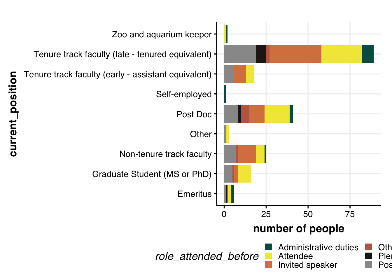

# to do:
# normalize the number of roles undertaken by a person in past IUSSI
# number of past roles / number of past IUSSI attended

The above plot might be misleading since the higher number of roles assumed by (activity of) late, tenured Profs might be due to the higher number of previous conferences attened by them. So, it might make sense to have a standardized metric that gives us a better understanding of the activity of each group in IUSSI.

Activity = number of roles assumed (including attendee) / number of IUSSIs attended

id <- character()
num_attended <- numeric()  
for (i in 1:length(levels(as.factor(dat$ID)))) {
    
    id[i] <- levels(as.factor(dat$ID))[i]
    
    num_attended[i] <-
      dat %>% 
      filter(ID == id[i]) %>%
      # select(which_attended_before)
      mutate(which_attended_before=as.character(which_attended_before)) %>% 
      pull(which_attended_before) %>% 
      unique() %>% 
      as.factor() %>% 
      levels() %>% length() %>% 
      as.numeric()
}

dummy.dat <- data.frame(ID=id, num_attended=num_attended)

## Add this information to the primary dataset

dat %>% 
  
  # add the num_attended column to dat
  left_join(dummy.dat, by="ID") %>% 
    # check to see if it worked
    # select(ID, which_attended_before, num_attended) %>% head(20)
  
  # remove the rows with no info
  filter(!is.na(role_attended_before)) %>%
  filter(!is.na(current_position)) %>%
  # filter(gender != "Other") %>% 
  
  select(ID, current_position, role_attended_before, num_attended) %>% 
    # head(20)
  
  distinct(ID, role_attended_before, current_position, num_attended) %>% 
  
  group_by(ID, current_position, num_attended) %>%
  summarize(num_roles = n()) %>% 
  arrange(as.numeric(ID)) %>% 
  
  # calculate activity
  mutate(activity = num_roles/num_attended) %>% 
    
  ## Plot: research_location + gender
  ggplot(aes(x=current_position, y=activity)) +
    # geom_bar(position="stack", stat="identity", size=2) +
    geom_boxplot(alpha=0.7, outlier.colour = "darkred", fill=viridis::inferno(10)[4]) +
    labs(y="# roles/attendance") +
    # geom_hline(yintercept = 5, col="grey60", alpha=0.7, size=1) +
    coord_flip() +
    theme_Publication() +
    scale_colour_Publication() +
    scale_fill_Publication() +
    # scale_fill_manual(values = roles.color) +
    guides(fill = guide_legend(nrow = 8)) +
    theme(legend.position = "none")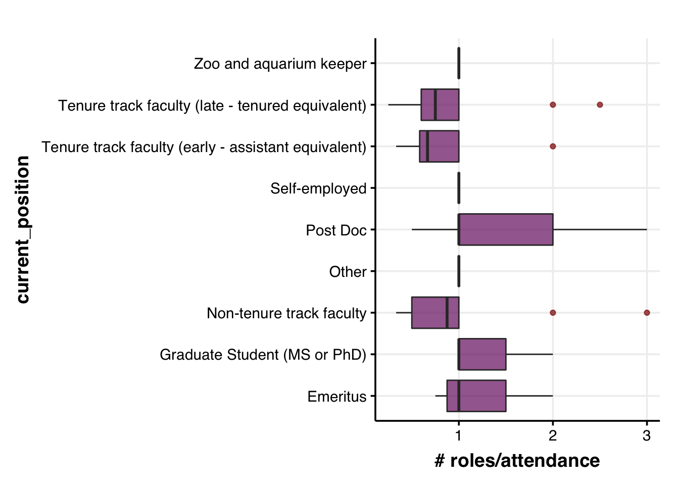

---

Role of attendee & ethnic identity

dat %>% 
  
  # remove the rows with no age/gender info
  filter(!is.na(role_attended_before)) %>%
  filter(!is.na(ethnic_identity)) %>%
  # filter(gender != "Other") %>% 
  
  distinct(ID, role_attended_before, ethnic_identity) %>% 
  group_by(role_attended_before, ethnic_identity) %>%
  summarize(num = n()) %>% 
    
  ## Plot: research_location + gender
  ggplot(aes(x=ethnic_identity, y=num, fill=role_attended_before, group=role_attended_before)) +
    geom_bar(position="stack", stat="identity", size=2) +
    labs(y="number of people") +
    # geom_hline(yintercept = 5, col="grey60", alpha=0.7, size=1) +
    coord_flip() +
    theme_Publication() +
    scale_colour_Publication() +
    scale_fill_manual(values = roles.color) +
    guides(fill = guide_legend(nrow = 3))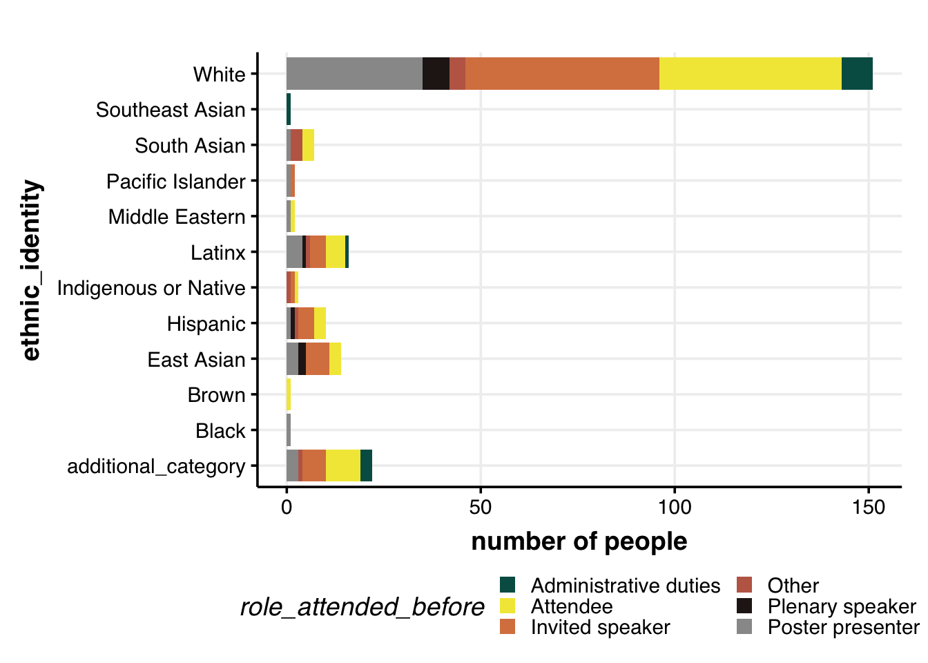

---

---

05 Over/Under-represented folks

Check which groups are over/under-represented at IUSSI, and for which activities.

#  load the GeneOverlap package to perform pairwise Fisher's exact test
library(GeneOverlap)

# which variable do you need to use for the x-axis
names.x <- c("gender", 
             # "age", 
             "residence_location", 
             # "research_location",
             # "current_position", 
             "ethnic_identity")

writeLines("Variables of interest:")

## Variables of interest:

writeLines(names.x)

## gender
## residence_location
## ethnic_identity

# initialize a list to hold all the possible groups that we want to plot
# on the x-axis
list.x <- list()
for (j in 1:length(names.x)) {
  
  # what are the different groups in the filtering column
  groups.x <- dat %>% 
  pull(names.x[j]) %>% 
  as.factor() %>% 
  levels()
  # what is the name of the filtering column
  var <- names.x[[j]]
  
  
  list.sub <- list()
  for (i in 1:length(groups.x)) {
    list.sub[[i]] <-
      dat %>% filter(.data[[var]] %in% groups.x[[i]] ) %>% pull(ID) %>% unique()
    names(list.sub)[i] <- groups.x[[i]] %>% as.character()
  }
  
  # Save the results for the filtering column and name the different lists
  list.x[[j]] <- list.sub
  
}

## DO THE SAME FOR THE Y-AXIS

names.y <- c("role_attended_before")
list.y <- list()

groups.y <- dat %>% 
  pull(names.y) %>% 
  as.factor() %>% 
  levels()
var <- names.y

list.sub <- list()
  for (i in 1:length(groups.y)) {
    list.sub[[i]] <-
      dat %>% filter(.data[[var]] %in% groups.y[[i]] ) %>% pull(ID) %>% unique()
    names(list.sub)[i] <- groups.y[[i]] %>% as.character()
  }
  
# Save the results for the filtering column and name the different lists
list.y <- list.sub


## Run the pairwise Fisher's tests ##

## What is the total sample size
nFolks <- dat %>% pull(ID) %>% unique() %>% length()

## Remove the groups that contain less than 5 individuals
list.y <- list.y[sapply(list.y, length)>=5]

for (i in 1:length(list.x)) {

  # remove for x
  list.x[[i]] <- list.x[[i]][sapply(list.x[[i]], length)>=5]
    
  if (i==4) {
    names(list.x[[i]]) <- names(list.x[[i]]) %>% str_sub(end=9)
    gom <- newGOM(list.y, list.x[[i]],
              nFolks)

  } 
  ## Let's perform the pairwise Fisher's exact test
gom <- newGOM(list.x[[i]], list.y,
              nFolks)
png(paste0(path_to_repo,
           "images/", folder.name,
           names.x[i],"_v_",names.y,"_gom.png"), 
    width = 30, height = 20, units = "cm", res = 300)
drawHeatmap(gom,
            # adj.p=T,
            cutoff=0.05,
            what="odds.ratio",
            # what="Jaccard",
            log.scale = T,
            grid.col="Oranges",
            note.col="black")
trash <- dev.off()

}

---

The goal is to perform enrichment analyses (using hypergeometric analyses) to identify under (or over) represented groups (based on gender, ethnicity, etc) in different activities (roles) at IUSSI.

We found several overrepresented groups for specific roles; we did not find any significantly underrepresented terms. The overrepresented groups in different IUSSI roles are shown in the table/figure below.

Results in a table

source(paste0(path_to_repo,"functions/underrepresentation_analyses.R"))

## Format the data
bg.dat <- 
  dat %>%
  select(ID, role_attended_before) %>%
  group_by(ID) %>%
  summarize(role_attended_before = str_c(role_attended_before, collapse = "; ")) %>%
  ungroup()
  
results.list <- list()
k <- 1
# get a list of all gender IDs
for (i in 1:length(list.x)) {
  
  names.vars <- names(list.x[[i]])
  
  for (j in 1:length(names.vars)) {
  results.list[[k]] <- 
      list.x[[i]][[j]] %>% 
        check_under(.,
                    bg.file = bg.dat,
                    what = paste0(names.x[[i]],": ",names.vars[[j]]),
                    atleast = 3)
  k <- k+1
  }
}

bind_rows(results.list, .id = "column_label") %>%
    dplyr::select(-column_label) %>% 
    as_tibble() %>% 
    filter(adj_pVal < 0.05) %>%
    mutate(adj_pVal = round(adj_pVal,3)) %>%
    filter(over_under=="over") %>% 
  
    filter(what_desc != other.var) %>% 
    filter(annot_term != "no_annot") %>% 
    
    select(annot_term:adj_pVal) %>% 
    arrange(annot_term, adj_pVal) %>% 
    
    DT::datatable()

---

And, here are the results as a heatmap.

Results as a figure

results.dat <- 
  bind_rows(results.list, .id = "column_label") %>%
    dplyr::select(-column_label) %>% 
    as_tibble() %>% 
    filter(adj_pVal < 0.05) %>% 
    mutate(adj_pVal = round(adj_pVal,3)) %>% 
    filter(over_under=="over") %>% 
  
    filter(what_desc != other.var) %>% 
    filter(annot_term != "no_annot") %>% 
    
    select(annot_term:adj_pVal) %>% 
    arrange(annot_term, adj_pVal)
  

mat <- 
  results.dat %>% 
  select(-over_under) %>% 
  pivot_wider(names_from = "what_desc",
              values_from = "adj_pVal",
              values_fn = list(adj_pVal = min)) %>% 
  as.data.frame() %>% 
  column_to_rownames("annot_term") %>% 
  as.matrix()


# Plot the matrix
### note: 
### make sure the library "plot.matrix" is loaded
### see here for more params: https://cran.r-project.org/web/packages/plot.matrix/vignettes/plot.matrix.html
png(paste0(path_to_repo,
           "images/", folder.name,
           "enrichement_results.png"), 
    width = 30, height = 20, units = "cm", res = 300)
par(mar=c(10.1, 16.1, 4.1, 6.1))
  mat %>% 
    t() %>% 
    plot(., 
         # border=NA,
         col=viridis::viridis(3),
         spacing.key=1.5,
         fmt.key="%.3f",
         xlab = "",
         ylab = "",
         axis.col=list(side=1, las=2), axis.row = list(side=2, las=1))
trash <- dev.off()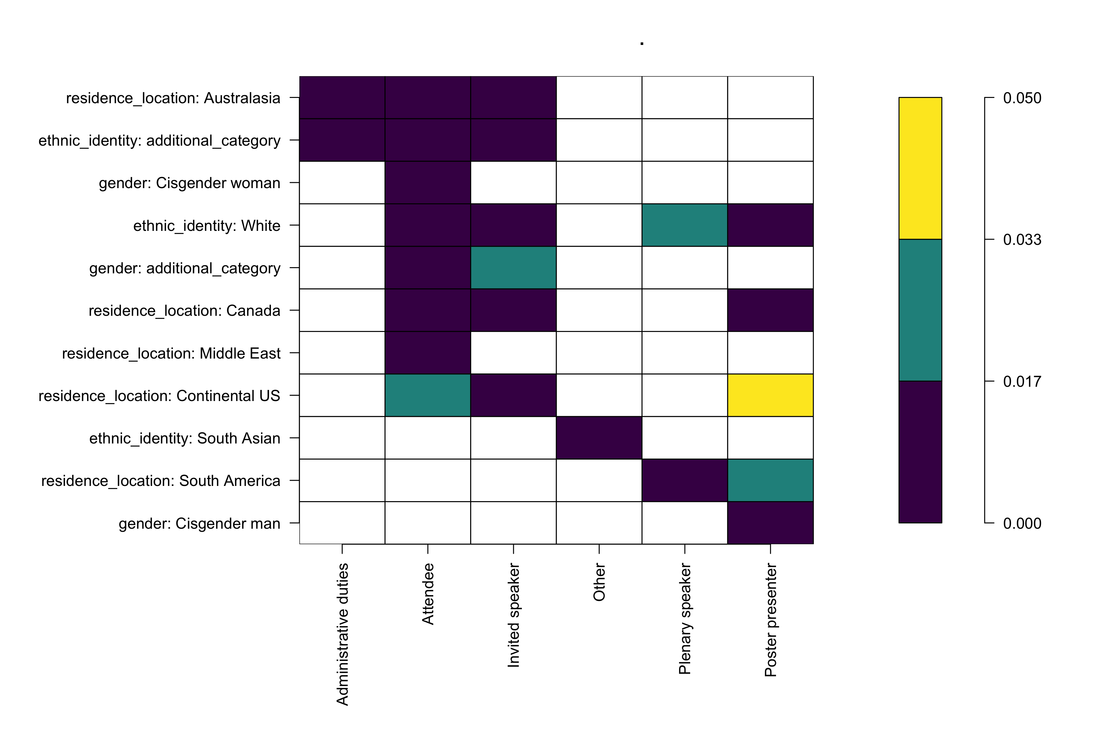

Results of the enrichment test; colors indicate p-values returned by the hypergeometric test. Lower p-values suggest possible over-representation.

So, what does the data tell us?

Write down the possible interpretations here. For example, the above figure tells us that

• Folks of ethnic_identity: white are overrepresented in most roles at IUSSI,

• Folks that relate to gender: Cisgender woman and residence_location: Middle East participate in IUSSI as attendees more than expected at random,

• and so on.

---

What next?

My thoughts: Once we, the committee, have all the summary statistics (and figures), and interpretations from the enrichment analyses, we should be ready to put together a brief document (pdf) for circulation. We might be able to highlight a few areas that we can improve on in the near future, and a few areas that we need to work on in the long-term.

---

Supplementary

1. Reproducibility

• All code used for this document is available on my Github.

• The function to perform enrichment analyses can be found here

2. IUSSI 2014 & 2018

A summary of the demography data for folks that attended IUSSI 2014 and 2018 can be found here.